CWPK #12: A Brief Pause to Learn Some Python

Let’s Get More Familiar with Python Syntax and Jupyter

Now that we have our basic environment set up and working, it is time to become a bit familiar with Python code and programs. To do so, we will use some online and reference documentation, relying in particular on an interaction environment with our Jupyter Notebook. In fact, from this point forward, all of our installments in the Cooking with Python and KBpedia series will also be accompanied by a working *.ipynb Notebook file that you are free to download and interact with at your leisure. Availability of the interactive notebooks will begin on Monday with CWPK #16.

Here are three interactive guides on how to program in Python using the interactive Jupyter Notebook environment. You may find use from all three (and there are many more on the Web, see especially GitHub and search on ‘jupyter python tutorial’, no quotes). I list these in suggested order for download and investigation if your time is limited:

1. An Introduction To Scripting in Python 3 – a good starting point with short, crisp lessons [1]
2. Python 3 Tutorial Using Jupyter Notebook – an update to Python3 from a well-regarded earlier Python2 guide [2]
3. An Introduction to Python and Programming – a 28-part notebook series. [3]

To download these from GitHub, go to the respective linked sites and pick the Clone or download button (1), followed by Download ZIP (2):

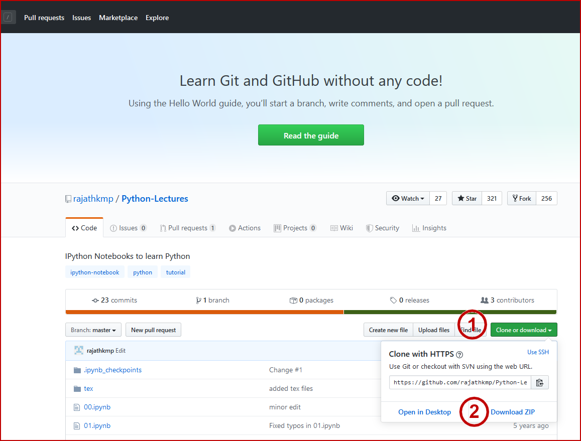
And save the *.zip files to a location of your choosing (see further below). (Recall we are punting on the question of GitHub ‘pull’ requests in this series.) Unzip the downloads to their respective directories. We are now ready to start the Jupyter Notebook.

Recall that we may launch the Jupyter Notebook from either the Anaconda Prompt (CWPK #11) or from the Anaconda Navigator (CWPK #10). If we are launching from the prompt, the command is (base) C:\Users\user\jupyter notebook. Upon launch we see the standard Jupyter Notebook entry screen using the default C:\Users\user\ location used by the program:

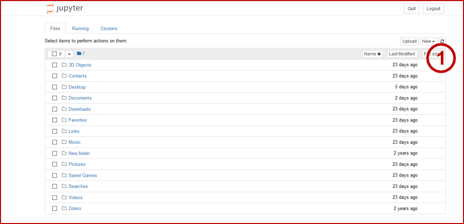
If you play around with that directory structure, you will notice that this default directory is the root, and you are unable to navigate above it in your local file system. That poses a problem for me personally. I have for years not accepted Microsoft’s attempt to steer all of my created documents into a directory structure of its choosing. I prefer being able to control where I store files directly. Since we will be downloading and using interactive notebook files throughout this CWPK series, right off the bat I do not like the idea of having to store these files in the Jupyter default directory.

So, I have three choices. One, I could download and place my files into a directory under this default directory. However, that does not solve my initial problem. Two, I could download the files somewhere directly on my local machine, and then use the Upload option (1) in Figure 1 to move them into this default directory. To do so, I invoke the Upload button, which pulls up the Window Explorer for file uploads to which I navigate to the directory where I had just unzipped the files. I then highlight the unzipped files of interest (note they all have the *.ipynb extension):

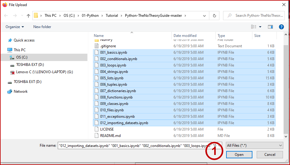
When I enter the Open button (1) that selects all of the files and returns me to the main Jupyter screen, as shown in Figure 4:

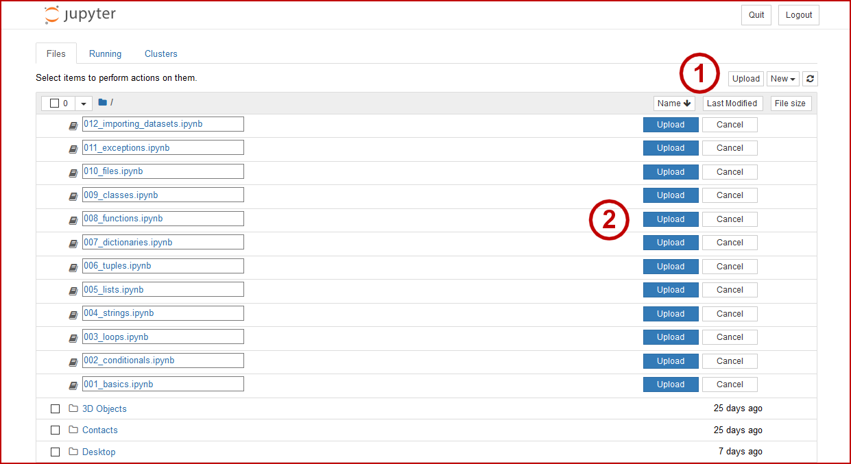
As I pick Upload for each selected file (2), the file gets copied to the default directory and the Upload row is then deleted. I continue this process until all of the selected files have been copied.

But this approach still ends up storing my notebook files in a location not of my choosing. If I were only going to poke at this application on rare occasions, perhaps that is OK. Yet my plan is to use notebook files aggressively. So that leads me to the third option of changing the location of the default directory.

There is a two-step process to do so, First, we need to go to the default directory and look for the .jupyter sub-directory (note the preceding period!), which should appear as C:\Users\user\.jupyter. We bring up the command window here and enter and run at the prompt:

jupyter notebook --generate-config

This command creates a new file, C:\Users\user\.jupyter\jupyter_notebook_config.py, which is populated with the various command switches that govern the Jupyter Notebook’s behavior. In its initial condition, this file does not exist, and all settings reflect initial defaults. Once this file is generated, it is now possible to overwrite these default settings. BTW, this file can subsequently be deleted, in which case Jupyter Notebook reverts to its factory settings.

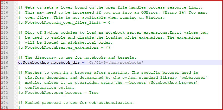
Open an editor for the jupyter_notebook_config.py and search for the following line in the file: #c.NotebookApp.notebook_dir = ''. It occurs about line 265 in the config file. Replace this text with your new desired starting root location for Jupyter. The entry should look like:

c.NotebookApp.notebook_dir = '/the/path/to/home/folder/'

When you make this update make sure you: 1) remove the # character at the beginning of the line and leave no space (the # designates the start of a comment line, and is thus not read at start-up time); 2) you use forward slashes in your path and do not use the tilde ~ character; and 3) you quote the file path in either matching single or double quotes. Figure 5 shows this modified config file for my own installation:

Once you complete the edits, save the file, and then re-start the Jupyter Notebook. Here we see the application now starts up at my preferred directory location:

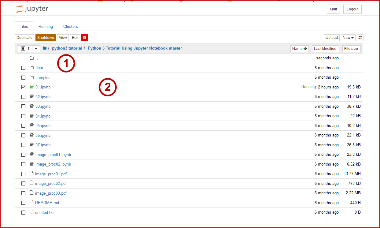
We can see we have a new directory structure (1). To open a Notebook page, we only need to double-click the entry (2) and we see that it is now running. Navigation through this tree file structure works as normally.

We will now select the second Notebook page on this list, 02.ipynb, and when we double-click it we get a new page in our browser with the new interactive page. Let’s explore some of the conventions of working with a Notebook page in Figure 7:

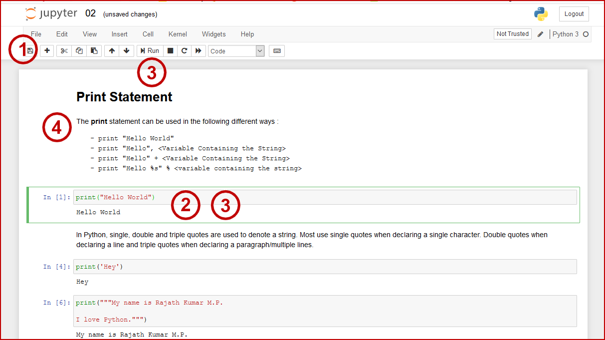
First, beside double-clicking, we may open and close Notebook pages using the old fashioned File option (1). Interactive areas of the Notebook page are shown as cells with the light gray background. The active interaction cell is bounded by the box with the margin highlight (2). To evaluate the cell in this active interactive we may either use the Run button or by using <shift>+<enter> when the cursor is in the active area (3). Also, the text on the page (4) may be entered or edited in the same way. We may either double-click or <shift>+<enter> when our cursor is in these text areas. Text entry occurs using a simple text formatting form called Markdown. We will be using Markdown aggressively throughout the rest of this series, and will have many occasions to describe its formatting and style options.

Like any document, existing Notebook pages can be loaded, modified, and saved again. This enables you to grab useful starting Notebooks on the Web, bring them into your own environment, modify them to reflect your own needs and circumstances, and then save them for later local use or for publishing to others. We can extend the active areas to include entire programs, with many complicated displays and activities possible in our Notebooks. This format is an excellent one for producing interactive dashboards and demos.

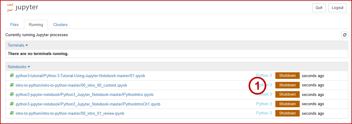
When we are done with our Notebook pages we may File → Close and Halt, Quit, which will stop the server and end all active pages, or use a Shutdown button for an individual page. As we shut individual pages, we are directed to a main screen that shows all of the Notebook pages currently active, which we may Shutdown directly (1) as Figure 8 indicates:

I encourage you to work through many of the examples provided in the three sources listed at the top of this article to gain a feel for Python syntax and the kinds of programming you can do with the language. The three sources at the beginning of this article proceed from simpler to more complicated within each source, and between sources, with the last example being the most comprehensive. The author of the last example suggests it takes about 90-120 hours to work through all of its examples [3]. Of course, simply browsing to gain a feel for the scope of the Python language can be done much quicker.

There are many online resources useful to Python programming. A simple Web search will turn up many Python learning scripts and examples. Here are some additional free ones I have found fairly useful:

• Interactive Python Tutorial from LearnPython.org
• Digital Ocean’s How to Code in Python3 Series
• Jupyter Notebook Tutorial from Google
• Jupyter Notebook Tutorial in Python from plotly (all tutorials in notebook form)
• Python Tutorial For Beginners – A Complete Guide
• Python3 Tutorial (see links in left-hand panel).

Endnotes: